Control Valve Sizing for Water Systems

The control valve can be sized to operate at a certain differential pressure by using a graph relating flowrate, pressure drop, and valve flow coefficients.

Alternatively, the flow coefficient may be calculated using a formula. Once determined, the flow coefficient is used to select the correct sized valve from the manufacturer's technical data.

Historically, the formula for flow coefficient was derived using Imperial units, offering measurement in terms of gallons/minute with a differential pressure of one pound per square inch. There are two versions of the Imperial coefficient, a British version and an American version, and care must be taken when using them because each one is different, even though the adopted symbol for both versions is 'Cv'. The British version uses Imperial gallons, whilst the American version uses. American gallons, which is 0.833 the volume of an Imperial gallon. The adopted symbol for both versions is Cv. The metric version of flow coefficient was originally derived in terms of cubic metres an hour (m³/h) of flow for a differential pressure measured in kilogram force per square metre (kgf/m²). This definition had been derived before an agreed European standard existed that defined Kv in terms of SI units (bar). However, an SI standard has existed since 1987 in the form of IEC 534 -1 (Now EN 60534 -1). The standard definition now relates flowrate in terms of m³/h for a differential pressure of 1 bar. Both metric versions are still used with the adopted symbol Kv, and although the difference between them is quite small, it is important to be certain or to make clear which one is being used. Some manufacturers mistakenly quote Kv conversion values without qualifying the unit of pressure differential.

Table 6.3.1 converts the different types of flow coefficient mentioned above: 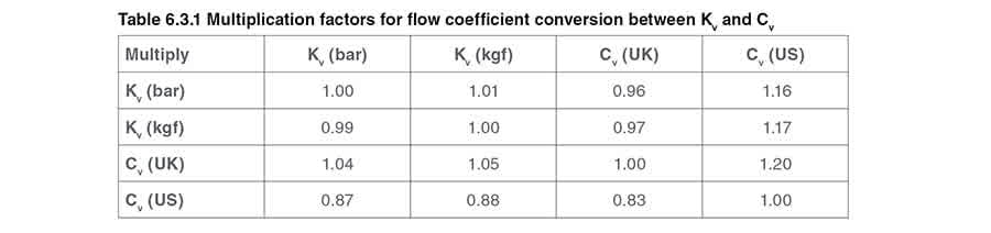For example, multiply Kv (bar) by 1.16 to convert to Cv (US).

The Kv version quoted in these Modules is always measured in terms of Kv (bar), that is units of m³/h bar, unless otherwise stated.

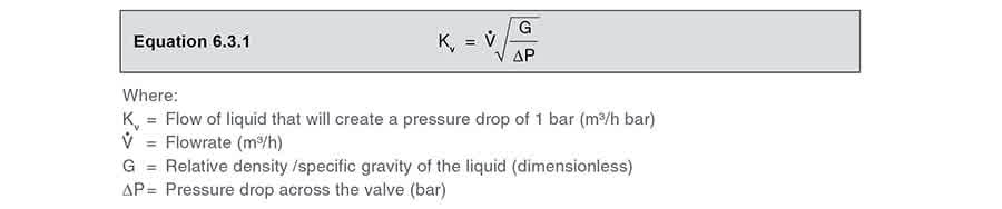
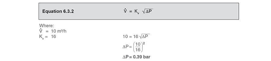
For liquid flow generally, the formula for Kv is shown in Equation 6.3.1. Sometimes, the volumetric flowrate needs to be determined, using the valve flow coefficient and differential pressure. For water, G = 1, consequently the equation for water may be simplified to that shown in Equation 6.3.2. 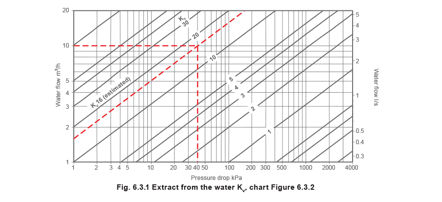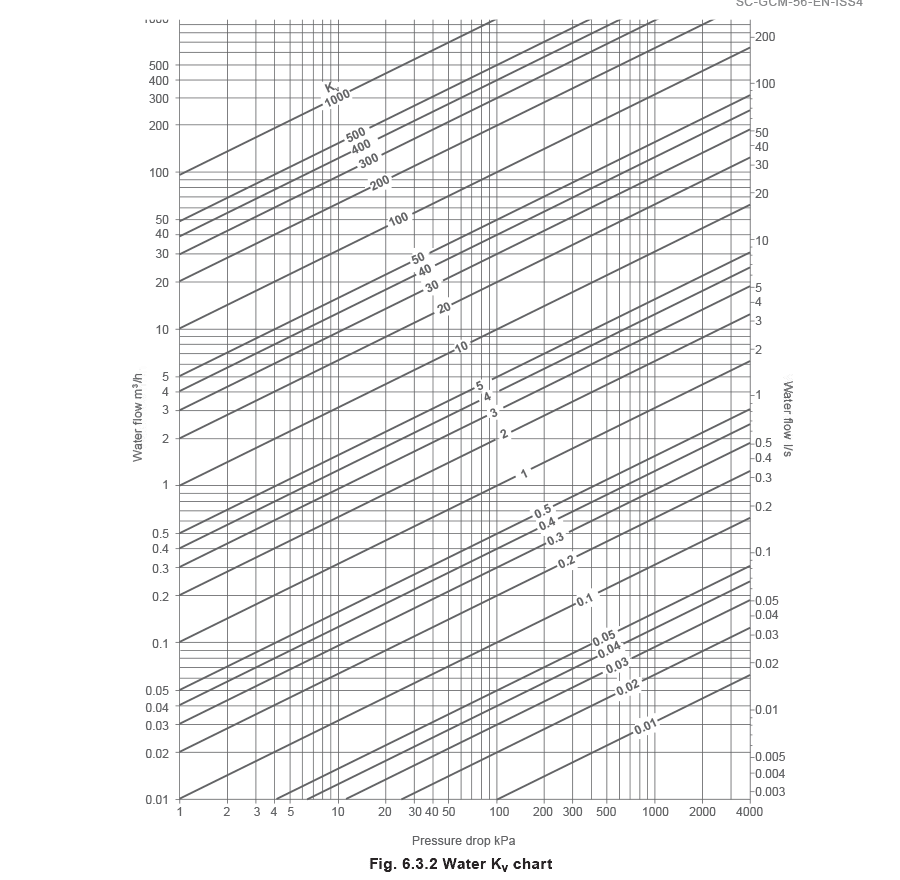Example 6.3.1 10 m³/h of water is pumped around a circuit; determine the pressure drop across a valve with a Kv of 16 by using Equation 6.3.2: Alternatively, for this example the chart shown in Figure 6.3.1, may be used. (Note: a more comprehensive water Kv chart is shown in Figure 6.3.2):

1. Enter the chart on the left hand side at 10 m³/h.
2. Project a line horizontally to the right until it intersects the Kv = 16 (estimated).
3. Project a line vertically downwards and read the pressure drop from the 'X' axis (approximately 40 kPa or 0.4 bar). Note: Before sizing valves for liquid systems, it is necessary to be aware of the characteristics of the system and its constituent apparatus such as pumps.

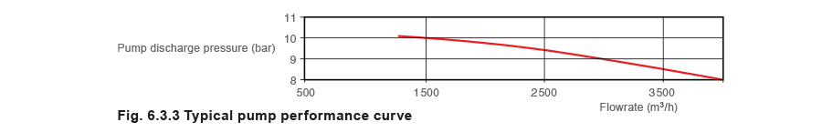
Pumps ****Unlike steam systems, liquid systems require a pump to circulate the liquid. Centrifugal pumps are often used, which have a characteristic curve similar to the one shown in Figure 6.3.3. Note that as the flowrate increases, the pump discharge pressure falls. Circulation system characteristics It is important not only to consider the size of a water control valve, but also the system in which the water circulates; this can have a bearing on which type and size of valve is used, and where it should be positioned within the circuit.

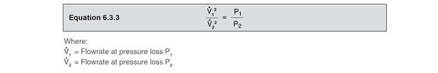
As water is circulated through a system, it will incur frictional losses. These frictional losses may be expressed as pressure loss, and will increase in proportion to the square of the velocity. The flowrate can be calculated through a pipe of constant bore at any other pressure loss by using Equation 6.3.3, where v̇1 and v̇2 must be in the same units, and P1 and P2 must be in the same units.are defined below. Example 6.3.2

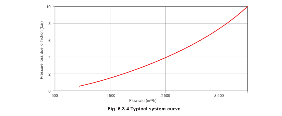
It is observed that the v̇1 flowrate through a certain sized pipe is 2500 m³/h when the pressure loss (P1) is 4 bar. Determine the pressure loss through the same size pipe (P2) if the flowrate v̇2 were 3 500 m³/h, using Equation 6.3.3. It can be seen that as more liquid is pumped through the same size pipe, the flowrate will increase. On this basis, a system characteristic curve, like the one shown in Figure 6.3.4, can be created using Equation 6.3.3, where the flowrate increases in accordance to the square law. 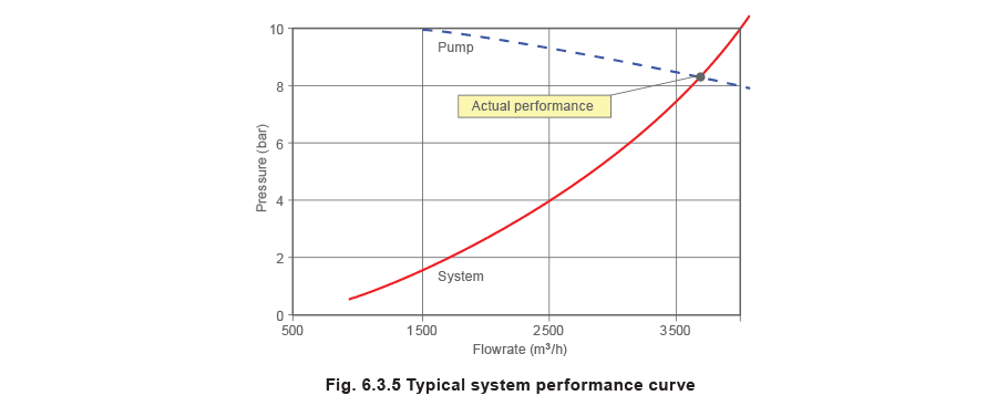Actual performance It can be observed from the pump and system characteristics, that as the flowrate and friction increase, the pump provides less pressure. A situation is eventually reached where the pump pressure equals the friction around the circuit, and the flowrate can increase no further.

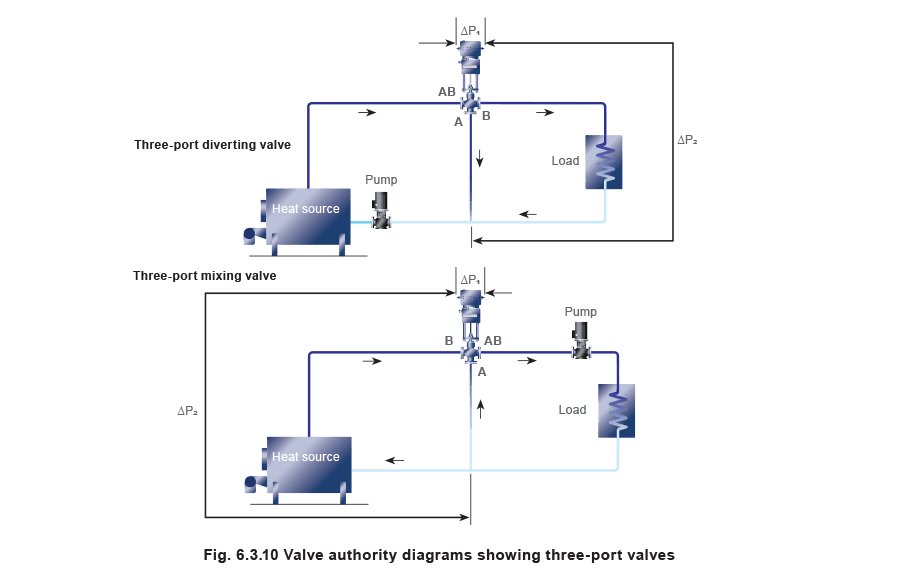
If the pump curve and the system characteristic curve are plotted on the same chart - Figure 6.3.5, the point at which the pump curve and the system characteristic curve intersect will be the actual performance of the pump/circuit combination. Three-port valve A three-port valve can be considered as a constant flowrate valve, because, whether it is used to mix or divert, the total flow through the valve remains constant. In applications where such valves are employed, the water circuit will naturally split into two separate loops, constant flowrate and variable flowrate.

The simple system shown in Figure 6.3.6 depicts a mixing valve maintaining a constant flowrate of water through the 'load' circuit. In a heating system, the load circuit refers to the circuit containing the heat emitters, such as radiators in a building. 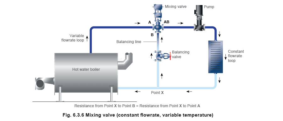The amount of heat emitted from the radiators depends on the temperature of the water flowing through the load circuit, which in turn, depends upon how much water flows into the mixing valve from the boiler, and how much is returned to the mixing valve via the balancing line.

It is necessary to fit a balance valve in the balance line. The balance valve is set to maintain the same resistance to flow in the variable flowrate part of the piping network, as illustrated in Figures 6.3.6 and 6.3.7. This helps to maintain smooth regulation by the valve as it changes position.

In practice, the mixing valve is sometimes designed not to shut port A completely; this ensures that a minimum flowrate will pass through the boiler at all times under the influence of the pump.

Alternatively, the boiler may employ a primary circuit, which is also pumped to allow a constant flow of water through the boiler, preventing the boiler from overheating.

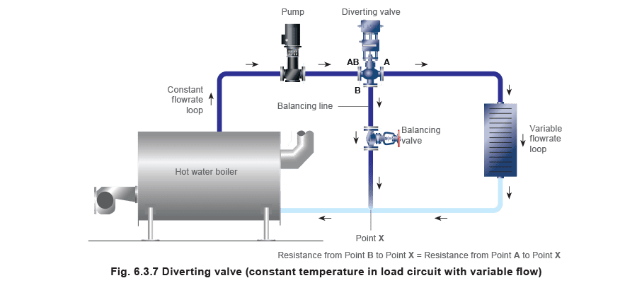
The simple system shown in Figure 6.3.7 shows a diverting valve maintaining a constant flowrate of water through the constant flowrate loop. In this system, the load circuit receives a varying flowrate of water depending on the valve position.

The temperature of water in the load circuit will be constant, as it receives water from the boiler circuit whatever the valve position. The amount of heat available to the radiators depends on the amount of water flowing through the load circuit, which in turn, depends on the degree of opening of the diverting valve. The effect of not fitting and setting a balance valve can be seen in Figure 6.3.8. This shows the pump curve and system curve changing with valve position. The two system curves illustrate the difference in pump pressure required between the load circuit P1 and the bypass circuit P2, as a result of the lower resistance offered by the balancing circuit, if no balance valve is fitted. If the circuit is not correctly balanced then short-circuiting and starvation of any other sub-circuits (not shown) can result, and the load circuit may be deprived of water.

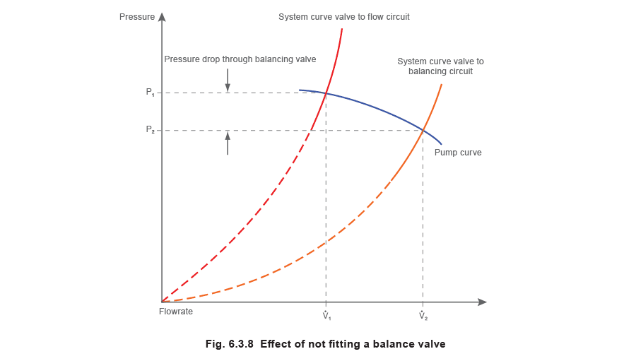
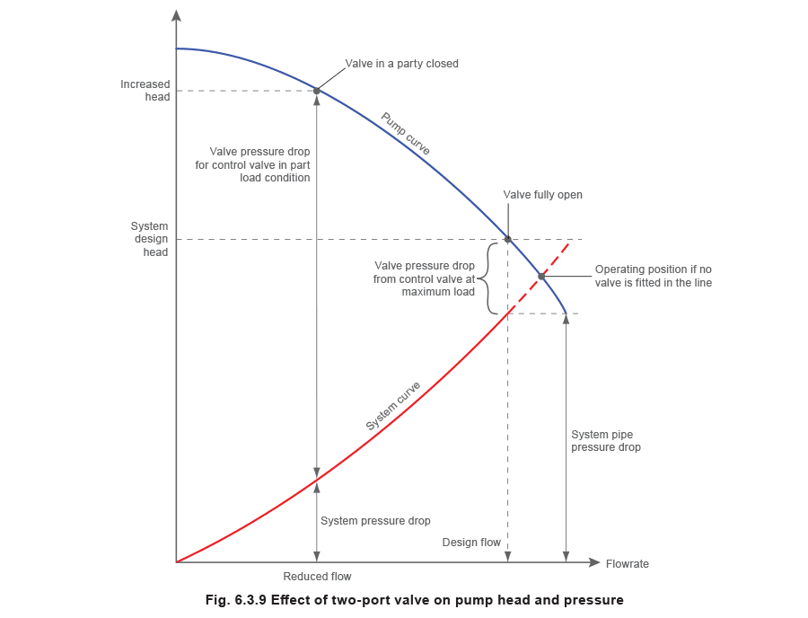
Two-port Valves When a two-port valve is used on a water system, as the valve closes, flow will decrease and the pressure upstream of the valve will increase. Changes in pump head will occur as the control valve throttles towards a closed position. The effects are illustrated in Figure 6.3.9.

A fall in flowrate not only increases the pump pressure but may also increase the power consumed by the pump. The change in pump pressure may be used as a signal to operate two or more pumps of varying duties, or to provide a signal to variable speed pump drive(s). This enables pumping rates to be matched to demand, saving pumping power costs.

Two port control valves are used to control water flow to a process, for example, for steam boiler level control, or to maintain the water level in a feedtank.

They may also be used on heat exchange processes, however, when the two-port valve is closed, the flow of water in the section of pipe preceding the control valve is stopped, creating a 'dead-leg'. The water in the dead-leg may lose temperature to the environment. When the control valve is opened again, the cooler water will enter the heat exchange coils, and disturb the process temperature. To avoid this situation, the control system may include an arrangement to maintain a minimum flow via a small bore pipe and adjustable globe valve, which bypass the control valve and load circuit.

Two-port valves are used successfully on large heating circuits, where a multitude of valves are incorporated into the overall system. On large systems it is highly unlikely that all the two-port valves are closed at the same time, resulting in an inherent 'self-balancing' characteristic. These types of systems also tend to use variable speed pumps that alter their flow characteristics relative to the system load requirements; this assists the self-balancing operation. When selecting a two-port control valve for an application:

• If a hugely undersized two-port control valve were installed in a system, the pump would use a large amount of energy simply to pass sufficient water through the valve. Assuming sufficient water could be forced through the valve, control would be accurate because even small increments of valve movement would result in changes in flowrate. This means that the entire travel of the valve might be utilised to achieve control.
• If a hugely oversized two-port control valve were installed in the same system, the energy required from the pump would be reduced, with little pressure drop across the valve in the fully open position. However, the initial valve travel from fully open towards the closed position would have little effect on the flowrate to the process. When the point was reached where control was achieved, the large valve orifice would mean that very small increments of valve travel would have a large effect on flowrate. This could result in erratic control with poor stability and accuracy.

A compromise is required, which balances the good control achieved with a small valve against the reduced energy loss from a large valve. The choice of valve will influence the size of pump, and the capital and running costs. It is good practice to consider these parameters, as they will have a bearing on the overall lifetime cost of the system.

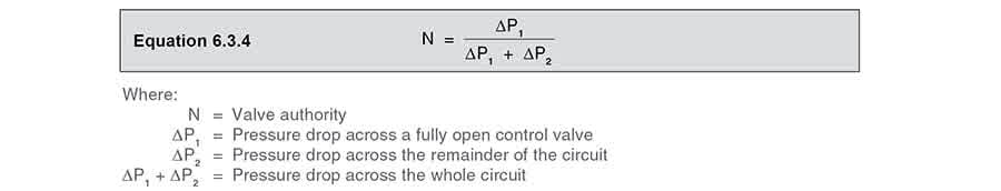
These balances can be realised by calculating the 'valve authority' relative to the system in which it is installed. Valve authority ****Valve authority may be determined using Equation 6.3.4. The value of N should be near to 0.5 (but not greater than), and certainly not lower than 0.2.

This will ensure that each increment of valve movement will have an effect on the flowrate without excessively increasing the cost of pumping power.power. Example 6.3.3A circuit has a total pressure drop ΔP1 + ΔP2 of 125 kPa, which includes the control valve.

a) If the control valve must have a valve authority (N) of 0.4, what pressure drop is used to size the valve?

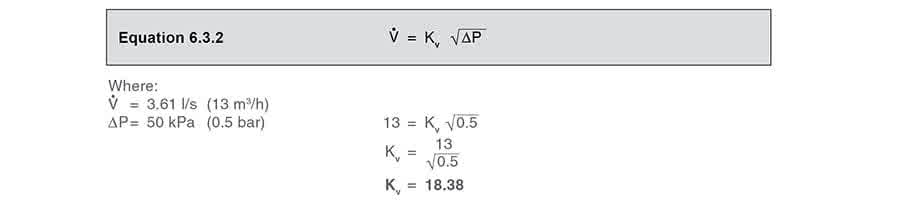
b) If the circuit/system flowrate v̇ is 3.61 l/s, what is the required valve Kv? Part a) Determine the ΔP 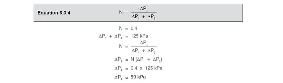Consequently, Δ P of 50 kPa is used to size the valve, leaving 75 kPa (125 kPa - 50 kPa) for the remainder of the circuit. Part b) Determine the Kv Alternatively, the water Kv chart (Figure 6.3.2) may be used. Three-port control valves and valve authority Three-port control valves are used in either mixing or diverting applications, as explained previously in this Module. When selecting a valve for a diverting application:

• A hugely undersized three-port control valve will incur high pumping costs, and small increments of movement will have an effect on the quantity of liquid directed through each of the discharge ports.
• A hugely oversized valve will reduce the pumping costs, but valve movement at the beginning, and end, of the valve travel will have minimal effect on the distribution of the liquid. This could result in inaccurate control with large sudden changes in load. An unnecessarily oversized valve will also be more expensive than one adequately sized. The same logic can be applied to mixing applications.

Again, the valve authority will provide a compromise between these two extremes.

With three-port valves, valve authority is always calculated using P2 in relation to the circuit with the variable flowrate. Figure 6.3.10 shows this schematically.